info@skybots.in
+91 8754531574
Location
| Introduction | 4.48 |
| UAV configuration + inertial VS body frame | 6.09 |
| Inputs and outputs of a 6 Degree of Freedom UAV drone | 3.31 |
| Propeller rotation directions 1 | 2.06 |
| Propeller rotation directions 2 - Helicopter example | 3.26 |
| 1st control action - Thrust | 3.51 |
| 2nd control action - Roll | 2.40 |
| 3rd control action - Pitch (exercise) | 1.11 |
| 3rd control action - Pitch (solution) + 4th control action - Yaw (exercise) | 2.15 |
| 4th control action - Yaw (solution) | 1.33 |
| Rotation vector direction | 3.59 |
| Clarification on measuring with respect to body or inertial frames | 0.48 |
| Global view of the drone's control architecture | 3.32 |
| Follow up! | 0.58 |
| Kinematics vs Dynamics | 3.48 |
| Measuring the UAV's position (exercise) | 2.31 |
| Measuring the UAV's position (solution) | 3.55 |
| Intro to describing attitudes 1 (exercise) | 3.36 |
| Intro to describing attitudes 2 (solution + new exercise) | 2.27 |
| 2D rotation matrix formulation (solution + new exercise) | 3.45 |
| From 2D to 3D rotations (solution + new exercise) | 2.25 |
| 3D rotation matrix formulation about the Z axis 1 (solution) | 1.47 |
| 3D rotation matrix formulation about the Z axis 2 (solution) | 2.02 |
| Projecting from 3D to 2D (exercise) | 3.12 |
| Projecting from 3D to 2D (solution) + constructing Rx and Ry matrices (exercise) | 3.45 |
| Constructing Ry matrix (solution) | 4.16 |
| Constructing Rx matrix (solution) | 2.39 |
| Orthonormal matrices (exercise) | 2.14 |
| Orthonormal matrices (solution) | 1.07 |
| 3D rotation sequence 1 (exercise) | 2.43 |
| 3D rotation sequence 2 (solution) | 8.30 |
| 3D rotation sequence - example (exercise | 12.36 |
| 3D rotation sequence - example (solution) | 5.28 |
| Intro to Euler angles (rotation about moving body frames) | 1.20 |
| Intuition on different conventions | 2.37 |
| Fixed VS Moving body frame rotations 1 (exercise) | 1.00 |
| Fixed VS Moving body frame rotations 2 (solution + new exercise) | 3.30 |
| Fixed VS Moving body frame rotations 3 (solution) | 7.42 |
| Rotation matrix conventions - Intro | 7.00 |
| Rotation matrix conventions - R_XYZ matrix product | 9.16 |
| Rotation matrix conventions - R_ZYX matrix product | 6.36 |
| Rotation matrix conventions - R_XYX matrix product | 4.44 |
| Rotation matrix conventions - R_XYZ vs R_ZYX example | 14.22 |
| Rotation matrix conventions - R_XYZ vs R_XYX example | 14.46 |
| Rotation matrix application to the UAV 1 | 3.32 |
| Rotation matrix application to the UAV 2 | 8.20 |
| Why is a special Transfer matrix needed 1 | 15.09 |
| Why is a special Transfer matrix needed 2 | 8.05 |
| Why is a special Transfer matrix needed 3 | 7.14 |
| Transfer matrix derivation 1 (exercise) | 7.12 |
| Transfer matrix derivation 2 (solution + new exercise) | 7.59 |
| Mathematical derivation of the Rzyx (moving frame) rotation matrix | 3.51 |
| Transfer matrix derivation 4 (solution) | 4.33 |
| Transfer matrix derivation 5 | 4.28 |
| Rotation & Transfer matrix application 1 - Kinematics wrap up | 5.14 |
| Rotation & Transfer matrix application 2 - Kinematics wrap up | 3.02 |
| Intro to Dynamics | 2.38 |
| Dot product 1 + Application | 5.08 |
| Dot product 2 +Application | 4.04 |
| Dot product 3 + Application (exercise) | 2.47 |
| Dot product 4 + Application (solution) | 3.54 |
| Cross Product 1 | 4.06 |
| Cross Product 2 (Exercise | 4.53 |
| Cross Product 3 (Solution) | 3.21 |
| Cross Product Application 1 | 7.19 |
| Cross Product Application 2 (exercise) | 2.25 |
| Cross Product Application 2 (Solution) | 3.44 |
| Mass moments of inertia & inertia tensor 1 | 5.18 |
| Mass moments of inertia & inertia tensor 2 (exercise) | 4.36 |
| Mass moments of inertia & inertia tensor 3 (solution) | 8.35 |
| Mathematical formulas of mass moments of inertia | 7.44 |
| Mathematical formulas of products of inertia | 3.09 |
| Principal axis | 3.33 |
| Mass moment of inertia applied to the UAV | 2.08 |
| Dynamics: Translational Motion (Inertial Frame) | 8.48 |
| Dynamics: Translational Motion (Body Frame) 1 | 9.11 |
| Dynamics: Translational Motion (Body Frame) 2 | 9.14 |
| Dynamics: Translational Motion (Body Frame) 3 | 7.31 |
| Angular momentum VS angular velocity 1 | 7.39 |
| Angular momentum VS angular velocity 2 | 3.30 |
| Dynamics: Rotational Motion (Inertial frame) | 10.40 |
| Dynamics: Rotational Motion (Body frame) 1 | 9.02 |
| Dynamics: Rotational Motion (Body frame) 2 | 3.28 |
| Autonomous vehicle lateral acceleration through new lenses | 20.03 |
| Dynamics: Rotational Motion (Body frame) - alternative form (exercise) | 3.53 |
| Dynamics: Rotational Motion (Body frame) - alternative form (solution) | 4.46 |
| From 6 DOF Newton-Euler to state-space (exercise) | 0.58 |
| From 6 DOF Newton-Euler to state-space (solution) | 11.29 |
| Applying Force of gravity to the UAV (exercise) | 9.02 |
| Applying Force of gravity to the UAV (solution) | 1.25 |
| Applying control inputs to the UAV (exercise) | 9.53 |
| Gyroscopic effect on a UAV - intuition 1 + control inputs (solution) | 4.06 |
| Gyroscopic effect on a UAV - intuition 2 (exercise) | 3.24 |
| Gyroscopic effect on a UAV - intuition 3 (solution) | 5.24 |
| Gyroscopic effect on a UAV - intuition 4 | 7.33 |
| Gyroscopic effect on a UAV - intuition 5 | 5.19 |
| Gyroscopic effect on a UAV - intuition 6 | 3.21 |
| Gyroscopic effect on a UAV - intuition 7 | 9.29 |
| Gyroscopic effect on a UAV - Math 1 | 7.27 |
| Gyroscopic effect on a UAV - Math 2 | 3.23 |
| From 6 DOF Newton-Euler to state-space - Math 1 (exercise) | 12.46 |
| From 6 DOF Newton-Euler to state-space - Math 2 (solution) | 13.02 |
| UAV plant model schematics 1 (exercise) | 9.04 |
| UAV plant model schematics 2 (solution) | 9.49 |
| Euler state integrator | 8.17 |
| Runge - Kutta integrator 1 | 11.02 |
| Runge - Kutta integrator 2 | 8.49 |
| Runge - Kutta integrator 3 | 8.37 |
| Runge - Kutta integrator 4 | 7.33 |
| Runge - Kutta integrator 5 | 3.03 |
| Runge - Kutta integrator 6 | 2.47 |
| Runge - Kutta integrator 7 | 5.22 |
| Runge - Kutta integrator 8 | 0.09 |
| From control inputs to rotor angular velocities - blade element theory 1 | 7.15 |
| From control inputs to rotor angular velocities - blade element theory 2 | 9.58 |
| From control inputs to rotor angular velocities - blade element theory 3 | 8.06 |
| From control inputs to rotor angular velocities - blade element theory 4 | 14.06 |
| From control inputs to rotor angular velocities - blade element theory 5 | 10.20 |
| From control inputs to rotor angular velocities - blade element theory 6 | 13.29 |
| From control inputs to rotor angular velocities - blade element theory 7 | 10.59 |
| From control inputs to rotor angular velocities - blade element theory 8 | 3.40 |
| From control inputs to rotor angular velocities - blade element theory 9 | 8.58 |
| From control inputs to rotor angular velocities - blade element theory 10 | 9.23 |
| From control inputs to rotor angular velocities - blade element theory 11 | 10.00 |
| From control inputs to rotor angular velocities - blade element theory 12 | 4.35 |
| From control inputs to rotor angular velocities - blade element theory 13 | 8.52 |
| Detailed recap 1: car & bicycle lateral equations of motion | 3.03 |
| Detailed recap 2: LTI state - space equations | 3.06 |
| Detailed recap 3: continuous VS discrete LTI | 3.23 |
| Detailed recap 4: system input calculation using Model Predictive Control | 5.10 |
| The global control architecture scheme - Intro | 5.53 |
| The elements of the sequential/cascaded controller | 3.17 |
| Different tasks of each sub-controller | 5.23 |
| The Planner | 8.10 |
| Stronger VS weaker dynamics 1 | 4.33 |
| Stronger VS weaker dynamics 2 | 12.28 |
| Reference trajectory equations in the planner | 13.22 |
| The affect of the control inputs on future states | 10.07 |
| Review of the global control structure | 3.12 |
| Review of the state space equations of the autonomous vehicle | 8.06 |
| The UAV's dynamics and kinematics equations revisited | 2.13 |
| Zero angle roll and pitch assumption 1 | 10.52 |
| Zero angle roll and pitch assumption 2 | 6.20 |
| Putting the state space equations in the Linear format 1 | 3.31 |
| Putting the state space equations in the Linear format 2 | 4.20 |
| Putting the state space equations in the Linear format 3 | 4.36 |
| Putting the state space equations in the Linear format 4 | 10.08 |
| Linear Parameter Varying form 1 | 10.18 |
| Linear Parameter Varying form 2 | 4.34 |
| Review of the steps from the equations of motion to the plant | 4.56 |
| The dimensions of the state space equation matrices | 4.30 |
| The dimensions of the state space equation matrices | 4.45 |
| Future state prediction formula 2: simplified LPV-MPC | 7.39 |
| Future state prediction formula 3: nonsimplified LPV-MPC | 13.22 |
| Future state prediction formula 4: nonsimplified LPV-MPC | 10.50 |
| Future state prediction formula 5: nonsimplified LPV-MPC | 8.07 |
| Cost function 1 - Review of the cost function components | 11.46 |
| Cost function 2 - Review on how to add extra states (augmentation) 1 | 7.17 |
| Cost function 3 - Review on how to add extra states (augmentation) 2 | 10.12 |
| Cost function 4 - review of the of the cost function Math - exercise | 7.41 |
| Cost function 5 - review of the of the cost function Math - solution | 3.24 |
| Cost function 6 - ignoring the constant terms in the cost function | 3.43 |
| Cost function 6 - ignoring the constant terms in the cost function | 6.25 |
| Cost function 8 - cost function in the matrix vector form 1 | 3.53 |
| Cost function 9 - cost function in the matrix vector form 2 | 5.29 |
| Cost function 10 - predicting future states | 15.49 |
| Cost function 11 - calculating the gradient of the cost function and the inputs | 8.43 |
| Extra: Nondiagonal MPC weights | 5.08 |
| Equations of motion for position control (inertial frame) - exercise | 7.22 |
| Equations of motion for position control (inertial frame) - solution | 7.22 |
| General feedback control architecture | 12.45 |
| Feedback Linearization Controller schematics - Part 1 | 4.04 |
| Differential Equations - intro | 5.51 |
| Differential Equations & the control law | 8056 |
| Solving differential equations - real roots 1 | 4.52 |
| Solving differential equations - real roots 2 | 12.15 |
| Solving differential equations - real roots 3 | 10.07 |
| Solving differential equations - complex roots 1 | 6.27 |
| Solving differential equations - complex roots 2 | 9.32 |
| Solving differential equations - complex roots 3 | 9.08 |
| Solving differential equations - complex roots 4 | 8.53 |
| Using the exponent for controlling a system - exercise | 4.53 |
| Using the exponent for controlling a system - solution | 8.45 |
| Poles & Laplace domain | 11.16 |
| From poles to differential equation constants - exercise | 8.17 |
| 5.36 | |
| From poles to differential equation constants - solution | 5.16 |
| From differential equations to state-space representation | 5.23 |
| Eigenvalues in control engineering & Determinants | 17.27 |
| Computing eigenvectors | 14.51 |
| Laplace VS Fourier frequency domain | 6.42 |
| Moving poles | 12.53 |
| Feedback Linearization Controller schematics - Part 2 | 3.55 |
| Simulation results with real & complex poles 1 | 8.08 |
| Simulation results with real & complex poles 2 | 15.47 |
| Simulation results with real & complex poles 3 | 15.18 |
| Feedback Linearization Controller schematics - Part 3 | 16.08 |
| Final Stretch - computing the final control inputs - Part 1 | 11.51 |
| Final Stretch - computing the final control inputs - Part 2 | 14.49 |
| Recommended reading: Great article about Kalman Filters | 0.10 |
| Intro to (Linux & macOS Terminal) & (Windows Command Prompt) | 12.54 |
| Python installation instructions | 12.54 |
| Python installation instructions - Windows 11 | 1.02 |
| Python installation instructions - Ubuntu | 5.14 |
| Installation of solver libraries - Ubuntu | 4.43 |
| Python installation instructions - macOS | 2.40 |
| Installation of solver libraries - MacOS | 8.04 |
| Simulation analysis & code explanation 1 - init function | 3.23 |
| General recommendation for tracking (autonomous car 2)9.33 | 4.41 |
| Simulation analysis & code explanation 2 - animation layout | 6.42 |
| Simulation analysis & code explanation 3 - adding a bit of drag 1 | 11.12 |
| Simulation analysis & code explanation 4 - adding a bit of drag 2 | 9.40 |
| Simulation analysis & code explanation 5 - exploring centripetal acceleration | 6.20 |
| Simulation analysis & code explanation 6 - exploring different trajectories | 10.51 |
| Simulation analysis & code explanation 7 - MAIN file 1 | 5.49 |
| Simulation analysis & code explanation 8 - trajectory generation + MAIN file 2 | 11.10 |
| Simulation analysis & code explanation 9 - correcting the units for ct & cq | 7.29 |
| Simulation analysis & code explanation 10 - position controller explanation | 11.21 |
| Simulation analysis & code explanation 11 - code for creating LPV matrices | 7.53 |
| Simulation analysis & code explanation 12 - extracting reference values | 18.31 |
| Simulation analysis & code explanation 13 - improving yaw motion | 2.25 |
| Simulation analysis & code explanation 14 - LPV-MPC function | 7.45 |
| Simulation analysis & code explanation 15 - plant function | 16.25 |
| Basic intro to Python animations tools | 12.12 |
| Simulation codes & course summary document | 1.27 |
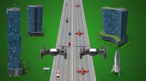
One of the greatest transformations that we will see in the next couple of decades is going to be the advent of autonomous drones. While being used extensively already, the applications of quadcopters will only grow in time. Drones will be used in delivery services, entertainment, medicine, military, rescue, structural quality inspection - places that people cannot reach easily, and in many other fields.
In many cases, there will be a predefined trajectory in a 3D space that the UAV needs to follow without human help. In fact, humans might simply give a simple command for the drone to go somewhere, and then, a specific trajectory will be generated by a computer in that direction and the UAV's control algorithms will need to determine EXACTLY how fast each rotor should turn in order to make the drone follow that trajectory with high-degree precision.
And that's what this course is all about - its about DESIGNING, MASTERING, and APPLYING these control algorithms together with deriving the dynamics equations for the quadcopter.
In this course, you will receive a full package when it comes to learning about how to model and control a UAV drone and make it follow a trajectory in a 3D environment. Not only you will learn how to model a UAV system mathematically by deriving the equations of motion using the principles of 3D Dynamics, but you will also be exposed to some of the most powerful control techniques out there such as Model Predictive Control and feedback linearization.
In 3D dynamics, you will learn the fundamental math and physics behind the UAV quadcopter drone modelling. You will learn how to describe the position and orientation of a UAV quadcopter drone in a 3D space using rotation and transfer matrices, Newton - Euler 6 Degree of Freedom equations of motion, widely used Runge - Kutta integrator in engineering and propeller dynamics.
In the end of the course, I will also explain to you the code in the Python simulator.
Understanding the material in this course fundamentally, being able to quantify it mathematically, and knowing how to apply it using coding - that will give you an advantage in your engineering career that you cannot even imagine yet. It will give you a competitive edge that you need in the labor market.

Mark Misin Engineering Ltd is an educational platform and engineering services provider led by instructor Mark Misin. The company specializes in teaching complex engineering concepts—such as Control Systems, Mathematical Modeling, and Python for Engineering—to help students and professionals bridge the gap between theory and real-world application.


Incorrect OTP
Incorrect OTP
Designed and Developed by B2L Mobitech Pvt. Ltd.
Incorrect OTP
Designed and Developed by B2L Mobitech Pvt. Ltd.